Briefly, we will also look at this example output from R, so you can again see how to obtain results from different software output. This will also let us examine an interaction plot to see whether we can visually see any interaction (again, it was found to be insignificant, so we shouldn’t really see any).
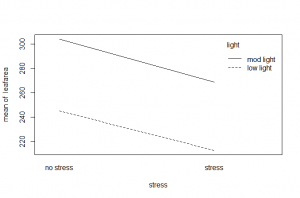
First, we visualize with the interaction plot. An interaction plot simply plots the mean of the response at each combination of factor levels and then connects the means with a line. We can see that the two lines (one for each level of light) are about the same distance apart, no matter what level of stress we are at. This indicates there does not appear to be interaction between the two factors.
Now, we look at the ANOVA table. The main difference is in how the rows are labeled. However, observation will reveal the exact same F-statistic, P-value pairs here as in the output above. Again, the ANOVA table is a common way to report these results, so this format is fairly standard between software packages.
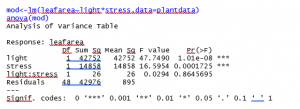
We can see that the interaction term is not significant (F=0.0294, P-value=0.8646). We would refit the model without the interaction term before doing post-hoc comparisons to identify the differences.
Here is the refit model.
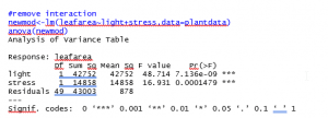
We see significance for both factor variables, so we run post-hoc comparisons. The example post-hoc comparison we will demonstrate is Tukey’s Honest Significant Difference (Tukey’s HSD). Again, in this context because there are only two levels for each factor, we don’t really need to do this. We know there are significant differences between the levels of light, and between the levels of stress in terms of average leaf area, simply because that is the only possible difference.
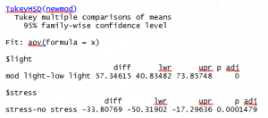
To identify differences looking at this output, you’d look at the p adj column, which are P-values for the difference comparisons adjusted to account for examining many comparisons at once. Both P-values are significant here, so both these differences are significant.