The following is a list of graphs that we will be using in this course.
Scatter plot
Use to display a numeric response variable with a numeric predictor variable. You may include different categories within your data. For instance, perhaps you want to look at the dispersal distance of black bears over time, with time as your predictor and distance as your response. You can use different colors or symbols to represent different groups of bears (e.g. red for females and blue for males, or triangles for juveniles and circles for adults).
Bar graph
Use to display count data, usually from a specific response variable. Can also incorporate information about categorical predictor variables. Alternatively, this plot can be used to display summary information from a continuous numeric response variable with a categorical predictor variable – usually the mean of the response and appropriate error bars are displayed for each level of the categorical predictor variable.
Box plot
Use to display a continuous numeric response variable with a categorical predictor variable. This is an alternative to the summary version of a bar graph and allows the viewer a better understanding of variation in the data.
Frequency Histogram
Shows how individuals are distributed along an axis of the measured variable. Frequency (the Y axis) can be absolute (i.e. number of counts) or relative (i.e. percent or proportion of the sample).
Briefly, let us look at an example of all these graphs in the context of an example, before learning to make each of them in Excel. These examples were all generated in a different software, called R. It is important to be able to recognize these graphs no matter what software was used to produce them.
Example
This data set contains information on abalones (sea snails). We are interested in being able to predict their age using physical measurements. Age is obtained by a procedure which involves staining and counting rings under a microscope. We explore various variables in the following graphs.
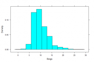
Due to our interest in predicting Age, we probably want to examine the distribution of Rings. This is a histogram of the variable Rings. We can see it has one peak (unimodal) with a tail off to the right side (right-skewed). The peak seems to be around 10 rings. The number of rings seems to range from 0 to 30.
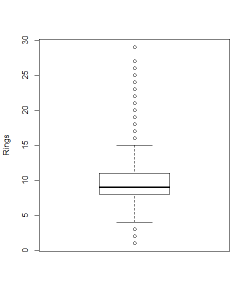
This is a boxplot of the variable Rings. We see many outliers (the dots) here. In fact, there may be many data points on top of each other at those points. The box itself shows us where the middle 50% of the data is. Here, we see 50% of the data lies between about 8 rings and 11 rings. The median seems to be 9 rings (where the middle bar is). The minimum is 1 ring and the maximum looks to be 29 rings. Observations with 3 or fewer rings or with 16 or more rings are flagged as outliers.
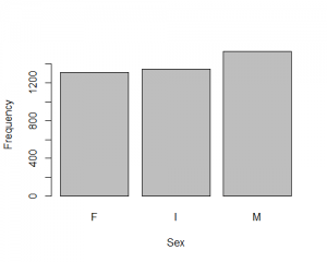
A variable that might impact our investigation is the Sex of the abalone. Here, in a barchart of the variable Sex, we can see that there were THREE levels of Sex recorded. The levels were Male, Female, and Infant. There appear to be more Males than Infants recorded, and more Infants recorded than Females.
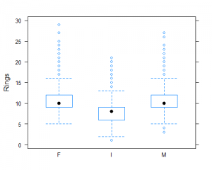
We can make a side-by-side boxplot to compare the Ring values across the Sexes. As expected, you can see the Infants have fewer rings than the Males and Females, at least comparing the medians. Typically for these plots, you can compare the medians (the black dots, middle bars, depending on the command used) and the variable spreads via the sizes of the boxes (this is called the Interquartile range). Here, the spreads all look very similar, and all groups have outliers.
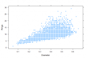
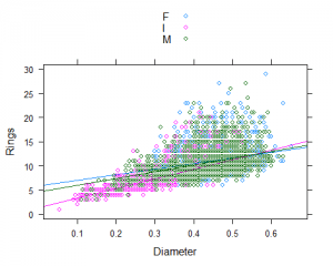
Finally, we know we want to use other variables in the data to try to predict Rings, so we should examine the relationship of Rings with those other variables. This is a scatterplot of Diameter (X) vs. Rings (Y). We see an overall linear pattern with positive association, but with increasing spread.
This plot could have a regression line added (you will learn about linear regression later this semester).
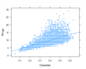
We could factor Sex into this plot by adding it as a grouping variable to the plot as well. Here, there are many data points, so the colors overlap and can make it hard to see the differences, but the idea is you can include different colors or symbols to denote different groups.