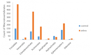
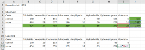
- Enter your data into a table in Excel. This is your ‘observed’ table. Graph your data.
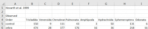
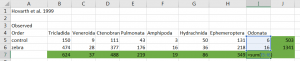
2. Calculate row totals, column totals, and overall total.
3. Next, you will create a table of expected values. This formula was explained in the previous example’s section.
To calculate the expected value: ![]()
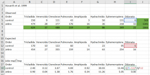
4. Now, you will calculate the (observed-expected)2/expected for each cell in your table. To do this, write an equation that collects the observed values from the original observed table that you entered and the expected values from the expected table that you created.
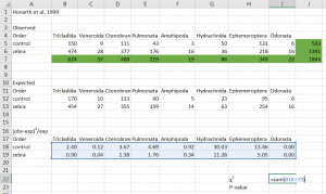
5. Next, to find the χ2 statistic, sum all the values in this new table.
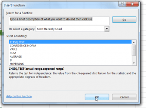
6. Now, go to the Formulas tab and select Insert Function.
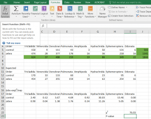
7. Select the CHISQ.TEST option.
8. Highlight your observed table for the “Actual_Range” and your expected table for “Expected_Range”. Click OK.
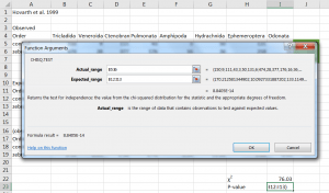
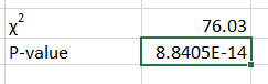
9. Now, you should have both a χ2 statistic and a P-value for your test.