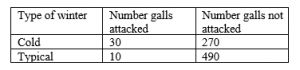
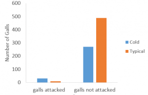
- Enter your data into a table in Excel. This is your ‘observed’ table. In statistics, we would call this a 2×2 contingency table, and the dimensions would change as the number of levels of each variable change. Graph your data.
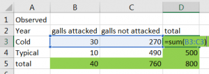
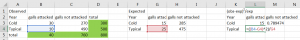
2. Calculate row totals, column totals, and overall total.
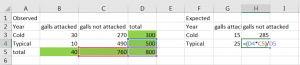
3. Next, you will create a table of expected values. These values represent what you would expect to see for each cell if the null hypothesis is true. This formula is called the cross-product rule. To understand the rule, consider the entry needed below for the last cell. We need the expected number of galls not attacked in the typical winter combination cell. Well, under the null hypothesis, the distribution of gall attacks is the same across both types of winter, so each row should have the same rate of no attacks as the overall rate. So, we look at the overall no attack rate (760/800, column total/overall total) and take that fraction of the number of Typical observations there are (500, the row total) to get the expected count for the cell. So, the computation was 500*760/800, which is the row total times column total divided by the overall total. In summary, to calculate the expected value:
![]()
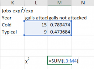
4. Now, you will calculate the (observed-expected)2/expected for each cell in your table. To do this, write an equation that collects the observed values from the original observed table that you entered and the expected values from the expected table that you created.
5. Next, to find the χ2 statistic, sum all the values in this new table. These pieces are called the components of the χ2 The cells with larger values (larger components) are the cells indicating a difference in distribution might be present there.
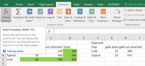
6. Now, go to the Formulas tab and select Insert Function.
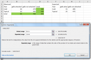
7. Select the CHISQ.TEST option. Note that this says it is the test for independence. It turns out that test is equivalent to the test for homogeneity, so this IS the correct option.
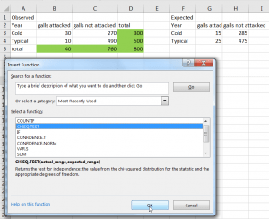
8. Highlight your observed 2×2 table for the “Actual_Range” (observed values–not the row/column totals) and your expected 2×2 table for “Expected_Range”. Click OK.
9. Now, you should have both a χ2 statistic and a P-value for your test.
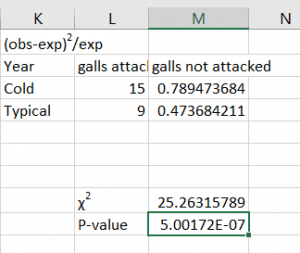
In this case, you reject the null hypothesis. There is a significant difference in bird predation by weather for this investigation (χ2=25.3, P<0.001).
10. Naturally, you will want to look for where the differences are if you have rejected the null hypothesis. Here, the idea is to look at the components of the χ2 Larger components are indicative of a difference. You can then look at the expected and observed counts for those cells to figure out if there were fewer or more observations than expected in those cells. Here, for example, we note that more galls were attacked than expected in the cold winter (and hence, also, fewer were attacked than expected during the typical winter).
This test is appropriate when the variables have more than 2 categories each as well. You just end up with larger tables. The process is the same, there are just more expected counts to compute and more components to add up for the χ2 statistic.