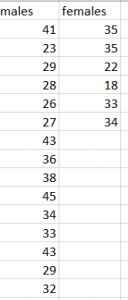
- Enter data into Excel.
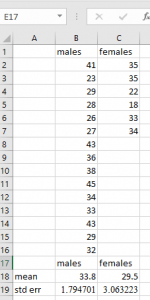
2. Compute the mean and standard error for each category.
Calculate standard error using: =(STDEV.S(cell:cell))/(SQRT(COUNT(cell:cell)))
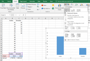
3. Highlight the means and insert a 2-D column graph.
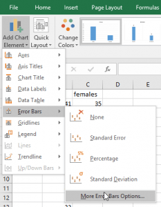
4. Click on the design tab and Add chart element. Select More Error Bars Options under Error Bars.
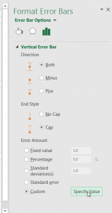
5. A new menu will show up on your right. Make sure the bars tab is selected. Select custom error bars and specify value.
6. Select your two values for standard error for both the positive and negative error values.
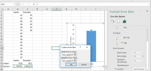
7. Click OK. Format.