Distributions

When we collect data on a random variable, there is typically a range of values in which that variable may fall. Certain values may be more common than others. To explore this pattern, we can construct a probability distribution, with values of the variable on the horizontal axis and probability of obtaining each value is on the vertical axis. Many statistical tests depend on the assumption of a specific type of distribution of the data or of the test statistic (with an assumption that the null hypothesis is true). We won’t go into detail about these distributions, except the normal distribution.

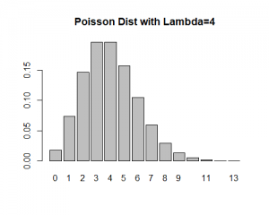
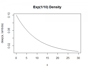
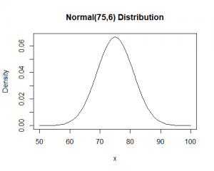
Here, we plot a few different distributions you might see working with biological data.

A Poisson distribution can arise from count data. The values are numeric, but discrete. There is a tail to the right.

An exponential distribution may be appropriate for numeric variables that are continuous with only positive values. This distribution also has a tail to the right.

 

Finally, you may observe a normal distribution. This is a distribution for numeric, continuous variables that has a bell-shaped distribution.

The normal distribution or Gaussian distribution is a distribution for variables that is often seen in biology. In the normal distribution, the majority of observations are found near the center (mean) of the distribution, with fewer observations as values move increasingly farther from the center. The distribution often applies for variables such as heights or weights. You may not always see this pattern for your variables though!

For bell-shaped distributions like this, there is a rough rule called the 68-95-99.7 Rule or Empirical Rule which states that 68% of values are within 1 standard deviation of the mean, 95% of values are within 2 standard deviations of the mean, and finally 99.7% of values are within 3 standard deviations of the mean. This rule is useful because it can help you understand how unusual a value is, if you standardize it by subtracting the mean and dividing by the standard deviation. For example, in the distribution above, the mean is 75 and the standard deviation is 6. The value of 81 is not unusual because (81-75)/6 = 1, so the value is exactly 1 standard deviation above the mean. The value of 51 however, is unusual because (51-75)/6 = -4, so 51 is four standard deviations below the mean.

The normal distribution is an important distribution in statistics because it has proven useful in statistical theory. It plays a role in some statistical test procedures, either in their theoretical development or in the conditions for the test procedure.